-
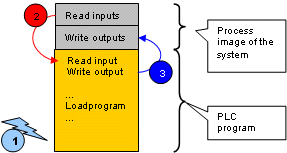
The input signal occurs shortly before the cycle change.
-
The inputs are copied to the process input image (within the update time).
-
The read signals are written to the process output image.
In the next cycle, the system writes the process image to the outputs.
Consequence:
The input signal can be directly detected and the mirrored signal can be output at the beginning of the next cycle.
-
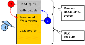
The input signal occurs approx. in the middle of the cycle.
-
After half a cycle has elapsed, the inputs are copied to the process input image (within the update time).
These signals are read in the user program. -
The read signals are written to the process output image.
In the next cycle, the system writes the process image to the outputs.
Consequence:
The input signal can only be detected half a cycle later and the mirrored signal is then also output later.
-
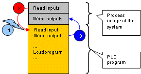
The input signal occurs shortly after the cycle change and after the system has read the inputs.
-
After a complete cycle has elapsed, the inputs are copied to the process input image (within the update time).
These signals are read in the user program. -
The read signals are written to the process output image.
In the next cycle, the system writes the process image to the outputs.
Consequence:
The input signal can only be detected after the current cycle has been completed. The mirrored signal can thus only be output after the end of the second cycle or before the beginning of the third cycle.
Time = load program + transmission time of the system (*)
Time = (time_min + time_max)/2
Time = 2 * load program + transmission time of the system (*)